Measuring heart rate with a smartphone camera
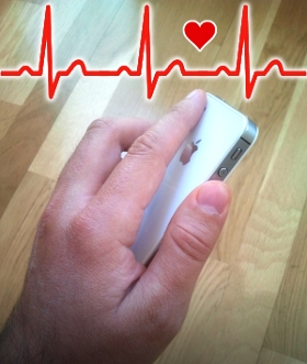 There are some apps out there that can read your heart rate with a smartphone camera. No need for external pulsometers. The procedure is simple: you press the smartphone camera lens gently with your finger and, after some seconds, a reading is shown. I was wondering how these apps were doing their magic and did some experiments to get a similar system working. In this post, a basic signal processing pipeline is discussed to estimate the heart rate evolution over time from a video sequence of a fingertip touching the camera lens. Continue reading to learn more or watch directly a quick video with the result.
It is time to open your photo app and observe what happens when you cover the camera with your finger. The frame is not black but slightly red. The ambient light is traveling through your finger tissues and is reaching the camera sensor. Despite the image looks like an almost static red frame (Fig. 2), the periodic oscillations of the blood flow in the vessels produce weak brightness variations that are undetectable for the naked eye, but can be discovered with signal processing.
The experiments in this post were done offline. I recorded the videos with an iPhone 4S and copied them to my laptop. Then, I processed them with Matlab. The full code is available here. Matlab has a very complete signal processing toolbox that makes life easier. However, you can use GNU Octave, too, and the code should be easy to port.
Heart beat monitor
Let's start our quest for the lost signal with a proposal for a simple processing pipeline in Fig. 1.

Fig. 1: Simple processing pipeline to extract the heart rate over time from a video sequence of the fingertip skin
1. Video signal acquisition
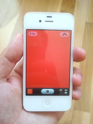 |
| Fig. 2: When the camera is covered with a finger, the naked eye sees a static red frame, but there are subtle variations caused by the blood flow under the skin that can be recovered processing the video signal. |
The first thing to take into account when it comes to sampling a signal is bandwidth. The normal human heartbeat is between 60 and 200 beats per minute (bpm), depending on age, fitness condition and the physical activity that the subject is doing. In my experiments, I have generously assumed that the target signal can be found between 40 and 230 bpm, i.e. 0.667 and 3.833 Hz. According to Nyquist, the sampling frequency should be at least twice the highest value (7.667 Hz) to catch the whole range of heartbeat frequencies without aliasing. With the iPhone 4S camera, the videos are recorded at 24 or 30 frames per second depending on the shot, which is more than 3 times the minimum.
2. Brightness signal computation
The signal we want to process is the brightness of the skin over time. We cannot ensure that all pixels in the image will contain the brightness variation that we are looking for and we want the rest of the processing pipeline to stay computationally light. Therefore, I chose to combine all pixels into a single average brightness value per frame. On the other hand, as I am thinking about implementing the algorithm in real time, I have skipped the common image brightness computation —combining the red, green and blue planes— in favor of a simple average of all the pixels in the red plane. This is computationally much cheaper and gives very similar results because almost all the image energy is in the red plane. So, the n-th sample of the red brightness function can be expressed as:
| b [n] | = |
|
Where:
W : width of the image in pixels
H : height of the image in pixels
v [n, x, y, 1] : light level of the red plane (index 1) at [x, y] coordinates of frame n in the video signal
In Matlab code, the red brightness signal can be computed with the following code snippet:
video = VideoReader('path to your video file here');

brightness = zeros(1, video.NumberOfFrames);

for i = 1:video.NumberOfFrames,

    frame = read(video, i);

    redPlane = frame(:, :, 1);

    brightness(i) = sum(sum(redPlane)) / (size(frame, 1) * size(frame, 2));

end
As the image size is constant over time and we are only interested in the shape of the signal, not in its amplitude, we could even omit the division by the total number of pixels. I am leaving it like that because it will later help visualizing the different spectrum peaks.
3. Band-pass filtering
After the signal acquisition, a band-pass filter attenuates frequencies outside the interest band. This reduces the noise in later processing steps (peak fine-tuning) and makes the resulting heart rate signal smoother. For our case, a second-order Butterworth filter is designed. The cutoff frequencies have been set to contain our band of interest: 40-230 bpm (Fig. 3). The Matlab code to design and apply the filter is:
BPM_L = 40;    % Heart rate lower limit [bpm]

BPM_H = 230;   % Heart rate higher limit [bpm]

FILTER_STABILIZATION_TIME = 1;    % [seconds]

% Butterworth frequencies must be in [0, 1], where 1 corresponds to half the sampling rate

[b, a] = butter(2, [((BPM_L / 60) / v.FrameRate * 2), ((BPM_H / 60) / v.FrameRate * 2)]);

filtBrightness = filter(b, a, brightness);

% Cut the initial stabilization time

filtBrightness = filtBrightness((v.FrameRate * FILTER_STABILIZATION_TIME + 1):size(filtBrightness, 2));
Notice how an initial piece of 1 seconds is cut off the filtered signal. It is an approximation of the time it takes for the filter to completely remove the constant signal offset (Fig. 3). If this initial piece is not removed, we might get bad readings of the heart beat during the signal stabilization time.
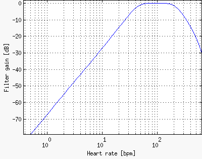
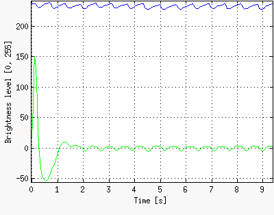
Fig. 3: On the left, the filter frequency response. On the right, original signal (blue) vs filtered signal (green). Notice the transient during the first second.
Other filter types can be tested. I chose Butterworth because:
- It is an IIR filter and the order required for a given bandwidth is much lower than with a FIR filter. Lower order usually means less computations.
- It has flat pass-band and stop-bands compared to other IIR structures that show ripples. This avoids favoring certain frequencies over others in the valid range.
4. Fast Fourier Transform
The Discrete Fourier Transform (DFT) is used to translate the signal from the time domain to the frequency domain. The Fast Fourier Transform (FFT) algorithm was used to save processing time when computing the DFT. While the computational complexity of the DFT is O(N2) for a set of N points, the FFT gets the same results with O(N · log2(N)), which means a huge speed-up when N is high.
There is a special command to compute the FFT in Matlab. The FFT of a real signal is a complex signal in which each complex sample represents the magnitude and the phase of the corresponding frequency. In our case, the phase is not needed. The FFT magnitude is easily computed in Matlab:
fftMagnitude = abs(fft(signal));
Sliding window
In order to give a continuous estimation of the heart rate, the FFT and the following two steps (peak detection and smoothing) are repeated every 0.5 seconds. This computation is always performed over a window containing the last 6 seconds of signal samples. Virtually, the window moves over the signal and this is why it is called "sliding" or "moving" window.
The 6-second length is not arbitrary. The window length directly affects frequency resolution and, thus, the accuracy of our estimation. The FFT of a signal sampled N times at a sampling frequency Fs is N bins long. All the bins together cover a bandwidth of Fs. So, the frequency difference between two consecutive bins is Fs / N. This is the frequency resolution (Fr). As the sampling frequency can be written as the number of window samples divided by the total time it took to sample them (the window time duration), we can say that:
| Fr | = |
|
= |
|
= |
|
Where:
Fr : frequency resolution
Fs: sampling frequency
N : number of window samples
Tw : window time duration
Therefore, the higher the window duration, the better the frequency resolution. The accuracy will be better, too, as it is half the resolution in this case.
However, increasing the window duration decreases the time accuracy. Think about the trivial case in which the whole signal length is picked as the window length. If a peak is detected in the FFT, it is impossible to tell when that tone started within the signal or how long it lasted. Whatever number we give will be a maximum of a window length away from the real value. Another problem of a long window is that it will force the user to wait for an equally long period to get a first reading after starting up the measurements.
In summary, with a 6-second window, we get a tolerable 6-second startup delay that gives a fair time accuracy of 6 seconds and a fair frequency accuracy of 5 bpm (half the FFT resolution). All in all, it looks like a good trade-off.
Why do we move the window in 0.5-second steps? Computing an estimate every 0.5 seconds does not improve the time accuracy of the output, but it increases the time resolution of the reading. It produces more heart rate output samples per second that will be later smoothed to provide a more continuous and frequent reading. With this, we are incrementing the time resolution of the reading but not its accuracy, which stays limited by the time resolution of the FFT.
Leakage reduction
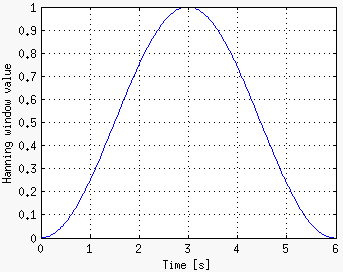 |
| Fig. 4: Hann window for the 6-second sliding window |
The DFT works ideally with infinite-time signals. A time-limited signal of length N is equivalent to multiplying its infinite-time counterpart by a rectangular signal of length N and amplitude 1. Frequency-wise, this results in convolving the infinite-time signal spectrum by the rectangular signal spectrum, producing leakage.
In order to reduce leakage, before computing the DFT, the input signal is multiplied by a function whose boundaries are zero. This forces the resulting boundary values to zero. The multiplying function is usually called "window". It must not be confused with the sliding window that we have talked about in the previous section. There are many window functions in the literature, each having their own virtues and disadvantages. I have particularly chosen the Hann window because it offers good resolution and good leakage rejection. Feel free to try others. There is a good comparative analysis of different window functions here.
In Matlab, the FFT magnitude for the sliding window with the Hann window can be computed with the following code. The result generated by the hann function is transposed because it is a column vector, while our signal is a row vector:
hannWindow = hann(size(slidingWindow, 2));

fftMagnitude = abs(fft(slidingWindow .* hannWindow'));
5. Peak detection
Once the FFT is computed for the current sliding window contents, magnitude peaks in the interest band are spotted thanks to the findpeaks function in Matlab. A sample is taken as a peak if it is either larger than its two neighbors or equal to infinity. Among the resulting peaks, the highest peak position is sought with the max function. Finally, it is translated to the corresponding frequency in the FFT vector:
% Translate the frequency range of interest to indices within the FFT vector

rangeOfInterest = ((BPM_L:BPM_H) / 60) * (size(fftMagnitude, 2) / samplingFrequency) + 1;

% Find peaks in the range of interest

[peaksValues, peakIndices] = findpeaks(fftMagnitude(rangeOfInterest));

% Find the highest peak

[maxPeakValue, maxPeakIndex] = max(peaksValues);

% Translate the peak index to an FFT vector index

bpmFreqIndex = rangeOfInterest(peakIndices(maxPeakIndex));

% Get the frequency in bpm that corresponds to the highest peak

bpmPeak = (bpmFreqIndex - 1) * (samplingFrequency / size(fftMagnitude, 2)) * 60;
6. Smoothing
At this stage, an approximate location for the most powerful tone in the frequency band has been found, but the possible outcomes are a discrete set in 10 bpm increments because of the frequency resolution produced by the 6-second window. We would like that the heart rate readings look more continuous, with 1 bpm frequency resolution instead. To achieve this, the signal window is correlated with a series of tones in phase and quadrature around the FFT peak in 1 bpm increments. The tones lie in the uncertainty interval around the peak caused by the FFT frequency resolution. The result of each signal-tone correlation is a complex number representing a phase-magnitude pair. The frequency that corresponds to the highest magnitude is taken as the smoothed heart rate:
| ck = |
|
bn e j 2π n ( fp - 0.5 Fr + k Fr') / Fs |
|
| HR = fp - 0.5 Fr + Fr' |
|
|ck | |
Where:
HR : Smoothed heart rate
bk : k-th sample of brightness signal
N : Window length in samples
fp : FFT peak frequency
Fr : FFT frequency resolution
Fr' : Smoothing frequency resolution
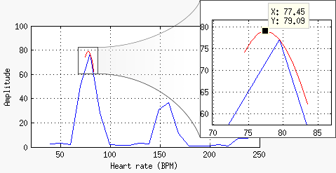
Fig. 5: Smoothing of an FFT peak. The DFT is computed on a zero-padded version of the signal in the window, but only within a range of FFT frequencies around the highest peak. The resulting DFT amplitudes form the red curve above the FFT, in blue. The frequency with the highest DFT amplitude, which is marked with the black square, is chosen as the current smoothed heart rate.
At first, I came up with this method intuitively, thinking of the correlation as a measure of similarity. My goal was to find the tone most similar to the signal in a frequency range around the FFT peak, regardless of the phase, by measuring the similarity (correlation) between the signal and a series of reference complex tones. In fact, it is what the FFT does, but using only orthonormal tones, whose period is an integer number of samples. Since the FFT frequencies are orthonormal, they constitute a base in which all signals can be expressed by linear combination. Correlating against other intermediate frequencies does not give more information because they themselves are formed by linearly combining the orthonormal ones. This is the reason why the result of this method is just smoothed FFT data, instead of higher accuracy extra information. Later, I realized that this method is equivalent to computing the FFT on a zero-padded version of the signal, which is a commonly used technique to smooth the FFT data, and picking only a frequency range. If the original 6-second signal in the window is zero-padded up to 60 seconds, the tone frequencies used in this method are found among the orthonormal frequencies of the 60-second FFT. Then, the method is equivalent to applying the DFT definition on the zero-padded window for certain frequencies only.
The advantage of this "zero-padding partial DFT" over the "zero-padding FFT" is speed. The FFT computes the result as a whole and cannot be divided to get subresults in a continuous frequency range; therefore, its complexity stays at O(Nz · log2(Nz)), where Nz is the length of the zero-padded window. On the other hand, the complexity of the proposed method is O(S · N), where N is the window length and S is the number of test tones. So, the complexity reduction factor (CRF) is:
| S = Fr / Fr' Fr' = Fs / Nz Fr = Fs / N |
|
⇒ S = Nz / N ⇒ S · N = Nz |
| CRF | = |
|
= |
|
= | log2(Nz) | = log2 |
|
Where:
CRF : Complexity Reduction Factor of the partial DFT method over the FFT on the zero-padded signal
Fs : Sampling frequency
Fr : Frequency resolution before smoothing
Fr' : Desired frequency resolution after smoothing
N : Window length
Nz : Zero-paded window length
S : Number of test tones
For a given sampling frequency, the higher the new frequency resolution, the more beneficial will be using the "zero-padding partial DFT" instead of the "zero-padding FFT". In our case, Fr' = 1/60 Hz and Fs = 24 Hz in the worst case. So, the CRF is approximately 10.5, which means that —roughly speaking— the time taken by the proposed method will be something in the order of a 10% of the time taken by the FFT on the zero-padded window.
Here is the Matlab code to implement the signal smoothing:
fftResolution = 1 / WINDOW_SECONDS;

lowFreq = bpmPeak / 60 - 0.5 * fftResolution;

smoothingResolution = SMOOTHING_RESOLUTION / 60;

testFreqs = round(fftResolution / smoothingResolution);

power = zeros(1, testFreqs);

freqs = (0:testFreqs - 1) * smoothingResolution + lowFreq;

for k = 1:testFreqs,

    re = 0; im = 0;

    for j = 0:(size(b, 2) - 1),

        phi = 2 * pi * freqs(h) * (j / samplingFreq);

        re = re + b(j+1) * cos(phi);

        im = im + b(j+1) * sin(phi);

    end

    % Since we only need to find the maximum, we can use power instead of magnitude and skip sqrt()

    power(k) = re * re + im * im;

end

[maxPeakValue, maxPeakIndex] = max(power);

smoothedBpm = 60 * freqs(maxPeakIndex);
Actively increasing the SNR
A good Signal-to-Noise Ratio (SNR) is essential to accurately detect the heart rate signal. It can be improved by either reducing the noise or increasing the signal power. In our case, the noise affecting the measurement comes from three sources basically:
- Image noise : It originates in the camera sensor. By averaging all the pixels for the brightness calculation, we are filtering out a big part of its spatial component. The band-pass filter that we are applying to the brightness signal is also rejecting much of its time component. However, there will always be some level of this noise in the band of interest.
- User behavior : The pressure variations of the fingertip against the camera lens may show up in the signal. If the user has shaky hands, it is better that she uses a finger of the hand holding the phone.
- Lighting changes : Since the finger is lit from behind, any change in the light sources or in the scene reflecting that light towards the camera may introduce noise in our pass band. For instance, moving the phone in the air while recording the video sequence may introduce artifacts if the scene parts in the field of view have very different light intensities.
Whereas the noise sources are obviously difficult to control —especially if the system is operated by someone else—, we can increase the signal level by illuminating the finger with a stable light source. If the smartphone has a torch that can be touched with the finger being recorded, it will light the tissues and improve the signal levels. However, if the torch is too powerful, it will saturate the image sensor and nothing but a pure white image will be recorded. If this is the case, try dimming the torch with your phone controls or covering it with a piece of fabric.
Results
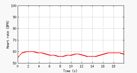
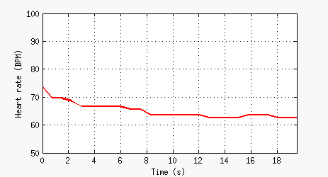
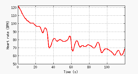
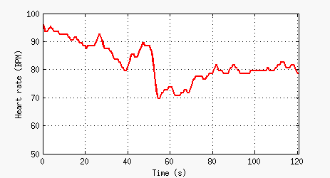
In order to check the system behavior, heart beat measurements with an iPhone 4S camera were performed on two individuals in two situations: at rest and after exercise (squats). Results are depicted in Fig. 6. Plots 6(a) and 6(c) correspond to a 34-year-old man who exercises regularly, whereas 6(b) and 6(d) belong to a woman of the same age who does not exercise. Besides having a lower resting rate, the active individual recovers faster than the sedentary one: >40 bpm vs <30 bpm decrements after the first minute, respectively.
Heart rates at rest were also estimated manually, by counting heart beats for one minute while videos were being recorded. The manual count results were 58 bpm for plot 6(a) and 67 bpm for plot 6(b), whereas the means computed from the measurements were 57.45 bpm for 6(a) and 65.09 bpm for 6(b).
|
|
Fig. 6: Heart rate over time for two people at rest (a, b) and recovering after squats (c, d). The curves (a) and (c) belong to a person who exercises often, while (b) and (d) belong to a person who does not. Exercise in (c) was longer and more intense than in (d). Heart rates at rest were manually estimated by counting heart beats for 1 minute while the video was being recorded. The manual count results were 58 bpm for (a) and 67 bpm for (b).
The following video shows an animation in 4x real-time of the case in Fig. 6(c) —active 34-year-old man recovering after intense squats—. Figure captions for Figs. 5 and 6 are applicable to the upper and lower plots in the video, respectively:


